NR 512 – Spatial Statistical Modeling
Exercise #2 – Introduction to Point Pattern Analysis in R
As discussed in class, a point pattern dataset contains a complete enumeration of events (i.e., objects of interest) occurring in a defined study region. These events could represent anything with a measurable location including trees, soil samples, animal nests, flower locations, crime occurrences, etc.
Point patterns have first-order properties, which are related to the intensity (i.e., density) of events across the study region, and second-order properties, which are related to the spatial dependence (i.e., spatial arrangement) of the events across the study area.

Objective: The goal of today’s lab is to learn some introductory spatial statistical approaches for characterizing first-order and second-order properties of a point pattern.
The datasets: Today you will be working with two separate point pattern datasets. The first dataset, called longleaf pine, is a marked point pattern containing locations and diameter measurements of longleaf pint trees in a southern forest. The second dataset, called bei, is a point pattern with location measurements of trees in a tropical rainforest. The bei dataset also contain a covariate containing topographical data. We will also be working with a .csv file called Lab3_longleaf.csv that contains the longleaf pine data. Save this file in a directory called lab3.

Exercise 1 – Becoming familiar with handling point patterns in spatstat
Today’s lab will be conducted using the spatstat package in R.
- Start R
- Load the spatstat package using:
> require(spatstat)
Note: You may need to download and install the spatstat package from CRAN if it is not installed on your machine. Ask the instructor or consult Lab 1 if you need assistance with this.
The spatstat package uses several classes of R objects to handle spatial data. In today’s lab we will be working with the planar point pattern (ppp) object class. The datasets we will be working with in today are automatically loaded into R when spatstat is installed.
- Examine the longleaf dataset. To do this you must first open the dataset in R by typing:
> data(longleaf)
We can examine the longleaf dataset by typing the following:
> longleaf
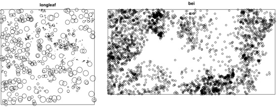
Based on the output we see that this is a marked planar point pattern with 584 events. We can also see that the marks are numeric values (as opposed to categorical) with double precision. The ppp object also contains information on the region (i.e., window) that contains the events. In this case it is a rectangle with an X coordinate range of 0-200 and a Y coordinate range of 0-200, with units in meters.
We can plot the longleaf ppp data by typing:
> plot(longleaf)
- Use the steps described above to examine the bei ppp object.
What type of object is bei? _______________________________________________________
How many events does bei contain? _______________________________________________
What is the size and area of bei’s window? __________________________________________
Plot bei and turn the plot in with your lab.
- Create a ppp object. The longleaf and bei datasets were automatically loaded into R when spatstat was installed, which is great. However, in the future you will be working with your own datasets, so learning how to create a ppp object from an external dataset will be a useful endeavor.
Use the read.csv command to read the Lab3_longleaf.csv file into R.
> ll_data <- read.csv(file = “INSTERT PATH AND FILE NAME HERE”, header = T)
explore the ll_data.
> names(ll_data)
We can see that the ll_data object has three columns, one containing the x coordinates, one containing the y coordinates, and one containing the diameter measurements.
> ll_data$diameter
To create a ppp object we need to use the ppp command in R. Look at the help file for the ppp command by typing:
> ?ppp
By examining the help file we see that the ppp command requires 4 types of information: x coordinates of each event, y coordinates of each event, window size (i.e., region size), and marks (i.e., values for each event). We can create a ppp object from the ll_data object by typing:
> ll_ppp = ppp(ll_data$x, ll_data$y, window=owin(c(0,200),c(0,200)), marks =
+ ll_data$diameter)
Note: Do not include the ‘+’ symbol at the beginning of the previous line, it just signifies that another line was needed to complete the command.
The above code sets the x and y coordinates for the ppp object to the x and y coordinates stored in the first two columns of the ll_data object. The window = owin portion of the command sets the x and y range of the window surrounding the point pattern, while the marks portion of the command assigns mark values to the ppp based on the diameter column in the ll_data object.
Plot the newly created ppp by typing:
> plot(ll_ppp)
Include this plot when you turn in today’s lab.
Exercise 2 – Characterizing first-order properties of a point pattern
In this portion of the lab we will use basic spatial statistical algorithms to characterize first-order properties of point patterns. As you will recall from lecture, first-order properties describe the way in which the expected value (mean or average) of the realized spatial stochastic process varies across the region (R). Spatial statistical algorithms for first-order analysis are used to characterize the intensity (i.e., density) of the point process across the region.
As you recall from lecture the overall intensity of a realized point process can be calculated via the following equation:
Equation 1:

Where λ is the intensity (or density), n is the number of events within R, and a is the area of R.
- Calculate the density of the longleaf dataset by extracting the number of events, calculating the area of the region (R) and plugging those numbers into equation 1.
> area.ll.r = longleaf$window$xrange[2] * longleaf$window$yrange[2]
The above code extracts the maximum x and y coordinates from the longleaf ppp object and uses them to calculate the area. It does this by accessing the window parameter of the object and asking it to report the second value in the x and y ranges characteristics.
What is the area of R? __________________________________________________________
What units is this in? __________________________________________________________
> n.ll.events = longleaf$n
The above code extracts the number of events from the longleaf ppp object.
How many events are in the longleaf ppp object? ____________________________________
Calculate the intensity by plugging these numbers into the above equation.
> lambda.calc = n.ll.events/area.ll.r
What is the overall intensity of events in the longleaf ppp object (remember to indicate units)? ___________________________________________________
The overall intensity could also be calculated automatically via a spatstat function by typing:
> lambda.auto <- summary(longleaf)$intensity
Or by typing :
> summary(longleaf)
What is the overall intensity of events in the longleaf ppp object according to this function (remember to indicate units)? ________________________
- Use one of the above approaches to calculate the overall intensity of the bei ppp object.
What is the overall intensity of the bei ppp object? _____________________
- Use quadrat counts to characterize the intensity of an inhomogeneous point process. Calculating the overall intensity of a point process may have some utility for comparing intensities of a portion process in different regions. However, a full characterization of first-order properties will require looking at how intensity changes, or varies, across a region.
Quadrat counts can be used as a starting point for characterizing an inhomogeneous point process. Quadrat counting employs the following steps:
– Divide the region into a series of equally sized quadrats
– Calculate the intensity of the point process in each quadrat (using equation 1).
Quadrat counting can be done in spatstat using the quadratcount command:
> data(longleaf)
> quadratcount(longleaf, nx = 4, ny = 4)
The above command divides the longleaf dataset in 16 equally sized square quadrats (4 in the x direction and 4 in the y direction) and returns a tally of the number of points in each quadrat as well as the size of each quadrat.
What is the number of events in the lower left quadrat? ________________________________
What is the area of each quadrat? __________________________________________________
Once we know the area of each quadrat the density of events within each quadrat can be calculated by typing the following:
> quadratcount(longleaf, nx = 4, ny = 4)/2500
What is the density of events in the lower right quadrat? ______________________________
We can also use plotting functions to explore the quadrat count output:
> Q <- quadratcount(longleaf, nx = 4, ny = 4)
> plot(longleaf, use.marks = F, cex = 0.5, pch = “+”)
> plot(Q, add = TRUE, cex = 2)
Include this graph when you turn in your lab.
Note: In the above command, plotting functions have been used to ignore the DBH measurements when plotting (use.marks = F). The cex and pch parameters are plotting controls for the size and type of symbol used, respectively.
The three lines above can be modified to plot quadrat density rather than the quadrat count:
> Q <- quadratcount(longleaf, nx = 4, ny = 4)/2500
> plot(longleaf, use.marks = F, cex = 0.5, pch = “+”)
> plot(Q, add = TRUE, cex = 2)
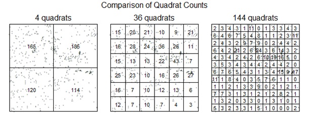
Challenge: Modify the code above to plot quadrat counts for 4 quadrats (2 in the x direction ad 2 in the y direction), 36 quadrats, and 144 quadrats. Try using the par() command with the mfrow=c(#row, #col) parameter to create a three column graph with the three plots in a row. It should look similar to:

Include these graphs when you turn in your lab.
What patterns do you observe when increasing and decreasing the number of quadrats?
____________________________________________________________________________________________________________________________________
- Use a kernel density estimator to characterize the intensity of an inhomogeneous point process. Quadrat counting is useful for characterizing the intensity of an inhomogeneous point process, however there are limitations including:
– The choice of origin, quadrat orientation, and quadrat size affects the observed frequency distribution.
– A significant amount of spatial data is lost.
KDE algorithms use a moving window approach to characterize intensity. This approach tends to preserve a greater amount of spatial detail and does not suffer as much from choices of origin, quadrat orientation, and quadrat size as compared to quadrat counting.
The density command can be used to run a KDE on a ppp object.
> den <- density(bei)
> plot(den)
Individual events can be added to the plot by typing:
> plot(bei, add = TRUE, cex = 0.5)
The density command uses a Gaussian operator to create a KDE estimate via the following equation:
Equation 2:

Where C(p,T) is the Gaussian kernel of bandwidth (i.e., radius) T centered at the location of interest p.
In the density command above bandwidth is calculated automatically using a ‘rule of thumb’. It defaults to 0.9 times the minimum of the standard deviation and the interquartile range divided by 1.34 times the sample size to the negative one-fifth power.
The bandwidth can be scaled via the sigma parameter within the density command:
> den <- density(bei, sigma = 10)
> plot (den)
Modify the density command to plot the density of the bei ppp object using the following bandwidths: 5, 10, 30, 70, 100, 200.
What influence does increasing and decreasing the bandwidth have on the density estimates?
____________________________________________________________________________________________________________________________________
Which bandwidth produces the best density estimate? ________________________________
Why did you pick this one? ______________________________________________________
Include a graph of the best density estimate when you turn in your lab.
- Compare the intensity of a point process to a covariate. Often, we want to know whether the intensity of points depends on the values of a covariate. For example, the tropical rainforest point pattern dataset bei comes with an extra set of covariate data bei.extra, which contains a pixel image of terrain elevation bei.extra$elev and a pixel image of terrain slope bei.extra$grad. It is of interest to determine whether the trees prefer steep or flat terrain, and whether they prefer a particular altitude.
Type the following to create a 2 x 2 matrix plot of the bei ppp object and slope:
> data(bei)
> slope <- bei.extra$grad
> par(mfrow = c(1, 2))
> plot(bei)
> plot(slope)
> par(mfrow = c(1, 1))
In the above plotting sequence, par() is a way defining parameters for a graphical object. Within this command, the mfrow parameter provides a way to slit the plotting area and is what let us plot two things side by side.
Include this graph when you turn in your lab.
In the quadrat counting example above, we used a series of equally sized quadrats to characterize the intensity of a ppp object. In quadrat counting methods, any choice of quadrats is permissible. From a theoretical viewpoint, the quadrats do not have to be rectangles of equal area, instead they could be regions of any shape. Quadrat counting is more useful if we choose the quadrats in a meaningful way. One way to do this is to define the quadrats using covariate information.
For the tropical rainforest data bei, it might be useful to split the study region into several sub-regions according to the terrain slope. This can be achieved via the following code:
> data(bei)
> Z <- bei.extra$grad
> b <- quantile(Z, probs = (0:4)/4)
> Zcut <- cut(Z, breaks = b, labels = 1:4)
> V <- tess(image = Zcut)
> plot(V)
> plot(bei, add = TRUE, pch = “+”)
The quantile command calculates the quartiles of the slope values with equal area (also referred to as a tessalation). In other words, we have divided the study region into four zones (quadrats) of equal area according to the terrain slope.
We can now use this quadrat to study the point pattern bei.
The command quadratcount also works with tessellations:
> qb <- quadratcount(bei, tess = V)
> qb
How many events are in each quadrat? _____________________________________________
The quadrats can be plotted by typing:
> plot(qb)
The text annotations show the number of trees in each slop region (slope increases with class number). Since the four regions have equal area, the counts should be approximately equal if there is a uniform density of trees.
Do the trees show any covariation with slope? ______________________________________
What trend do you see? _________________________________________________________
Include this graph when you turn in your lab.
We can also use a similar approach leveraging KDE intensity estimates to determine if the intensity of the point process is a function of some covariate (Z).
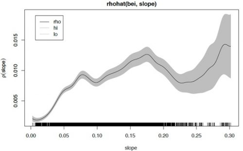
> plot(rhohat(bei, slope))

The plot is an estimate of the intensity as a function of terrain slope z. It indicates that the Beilschmiedia trees are relatively unlikely to be found on flat terrain (where the slope is less than 0.05) compared to steeper slopes. The black line (rho) is the intensity estimate and the grey region represents confidence limits.
