NR 512 – Spatial Statistical Modeling
Exercise #4 – Modeling Point Patterns in R
Quadrat Counts, F-, G-, K-, and L-functions
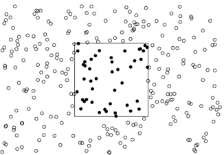
As discussed in class, a point pattern dataset contains a complete enumeration of events (i.e., objects of interest) occurring in a defined study region. These events could represent anything with a measurable location including trees, soil samples, animal nests, flower locations, crime occurrences, etc.

Point patterns have first-order properties, which are related to the intensity (i.e., density) of events across the study region, and second-order properties, which are related to the spatial dependence (i.e., spatial arrangement) of the events across the study area.
Objective: The goal of today’s lab is to learn how to use a Poisson process to model first-order properties (quadrat counting) and second-order properties (F-, G-, K-, and L-functions) of a point pattern. Remember, first-order properties are related to the density or intensity of the point process while second-order properties are related to the interdependence among events.
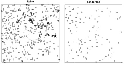
The datasets: Today you will be working with two separate point pattern datasets. The first dataset, called longleaf, is a marked point pattern containing locations and diameter measurements of longleaf pine trees in a southern forest. We are not interested in the marks for this lab, so one of the first steps is to create a new ppp object without marks. The second dataset, called ponderosa, is a point pattern with location measurements of ponderosa pine trees in a western forest.

Exercise 1 – Testing for CSR with quadrat counts
Today’s lab will be conducted using the spatstat package in R.
- Start R
- Load the spatstat package:
> require(spatstat)
We will be working with the longleaf dataset, which is a marked point pattern because there are tree diameter measurements for every event. We are not interested in the marks for this lab, so first step is to create a new ppp object without the marks. Type the following:
> data(longleaf)
> llpine <- ppp(longleaf$x, longleaf$y, window = longleaf$window)
This line of code uses the ppp command (which was discussed in lab 3) to create a new ppp object (called llpine) that only contains the x and y coordinates and analysis window from the longleaf dataset.
- Examine the llpine dataset. We can examine the longleaf dataset by typing the following:
> llpine
Based on the output we see that this is a marked planar point pattern with 584 events. The ppp object also contains information on the region (i.e., window) that contains the events. In this case it is a rectangle with an X coordinate range of 0-200 and a Y coordinate range of 0-200, with units in meters.
We can plot the longleaf ppp data by typing:
> plot(llpine)
The next series of steps demonstrate how to use quadrat counts to test for CSR. Remember, Quadrat Counts are a method of point pattern analysis in which the study region is sampled using a set of similar shapes (quadrats) and the number of events in each quadrat is counted. Analysis of the resulting quadrat counts can help determine whether the pattern is evenly spaced or clustered. Quadrat analysis may be based on a set of randomly located quadrats (common in fieldwork) or on a census where the quadrats fill the study regions without overlaps.
As you will recall from lecture, the homogeneous Poisson process (CSR) is usually taken as the appropriate ‘null’ model for a point pattern. Our basic task in analyzing a point pattern is to find evidence against the CSR hypothesis.
A classical test for the null hypothesis of CSR is a Chi-square test based on quadrat counts. As you can recall from lecture, a Poisson distribution can be used to calculate the expected number of events on a quadrat by quadrat basis as a function of the intensity of the process. This expected number of events per quadrat is compared to the observed number of events per quadrat to test for CSR.
The quadrat test command can be used in spatstat to test for CSR using quadrat counting:
> quadrat.test(llpine, nx = 3, ny = 3)
This command returns the results from a chi-square test comparing observed quadrat counts to theoretical quadrat counts under a Poisson process. In this case 9 quadrats were used (i.e., a 3×3 grid).
Based on this analysis do you reject or fail to reject the hypothesis of CSR? Why or Why not?
______________________________________________________________________________
______________________________________________________________________________
______________________________________________________________________________
Report the Chi-square and p-value: _________________________________________________
You can also visualize the results by typing the following:
> plot(llpine)
> plot(quadrat.test(llpine, nx = 3, ny = 3), add = T, cex = 2)
The resulting graph displays the event locations, quadrats, and text for observed counts (upper left text), expected counts (upper right text), and residuals (lower center text).
Include this graph when you turn in today’s lab.
Saving Plots: There are many ways to save plots, one such example follows:
> setwd(“FOLDER PATH”)
> dev.copy(tiff, “FIGURE_NAME.tiff”, units = “in”, width = 10, height = 10.68, res=300,
+ compression = c(“none”))
> dev.off()
In this example, the setwd() allows you to define the location you want to save the figure to, dev.copy() allows you to name the figure and define its dimensions, and the dev.off() ends the commands so that you do not over right the figure you created.
Use the methods and code above to use quadrat counting to test for CSR on the ponderosa using a 4 X 4 quadrat grid.
Based on this analysis do you reject or fail to reject the hypothesis of CSR for the ponderosa dataset? Why or Why not?
____________________________________________________________________________________________
____________________________________________________________________________________________
____________________________________________________________________________________________
Report the Chi-square and p-value: _________________________________________________
Create a plot to visualize these results (similar to the plot for the longleaf pine dataset). Turn in this plot with your lab.
Exercise 2 – Testing for CSR with G-, F-, K-, and L-functions
In this exercise, you will use distances between events or between events and points to test for CSR based on second-order properties.
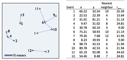
The G-function is a function in point pattern analysis based on the cumulative frequency of the shortest inter-event distances between events in a point pattern.

In spatstat, the Gest command can be used to test for CSR using the G-function:
> Gllp = Gest(llpine)
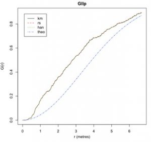
> plot(Gllp)

The command above produces a graph that plots the empirical and theoretical G-functions. The X-axis is distance and Y-axis is the G-function. The blue line represents the theoretical G-function under a Poisson process. The black, red, and green lines represent empirical G-functions calculated using different border correction techniques (these will be discussed in a later lab).
When interpreting this graph remember that empirical G values greater than theoretical G values indicate clustering in the dataset, while empirical G values less than theoretical G values indicate regular patterns in the dataset.
Based on this graph does the longleaf dataset follow the CSR hypothesis? Why or Why not?
______________________________________________________________________________
______________________________________________________________________________
The question to ask at this point is if this departure is statistically significant. As discussed in class, Monte-Carlo simulations can be used to generate confidence intervals around the theoretical G-function.
Monte-Carlo simulation (or method): A statistical method of generating a sampling distribution for a statistic, usually in the absence of a well understood analytically derived method. In spatial analysis it is often difficult to derive expected distributions of statistical measures, so Monte-Carlo simulation is often used. Based on an understanding of the processes at work in generating the spatial data under analysis, a computer simulation is used to generate a number of synthetic datasets, which are then analyzed using the measure under test. The results from multiple synthetic datasets provide a synthetic sampling distribution against which observed measurements can be assessed.
To perform a Monte-Carlo simulation type:
> G.Env.llpine <- envelope(llpine, Gest, nsim = 39, rank = 1)
> plot(G.Env.llpine)
The grey region plotted around the theoretical G-function corresponds to upper and lower confidence intervals generated from 39 Monte-Carlo simulations (nsim = 39).
Based on this graph, does the longleaf dataset display a significant departure from the CSR hypothesis? Why or Why not?
______________________________________________________________________________
______________________________________________________________________________
Similar approaches can be used to run the F-, K-, and L-functions in spatstat using the Fest, Kest, and Lest commands, respectively.
F-function: A function in point pattern analysis based on the cumulative frequency of the shortest distance between events in a point pattern and a set of randomly placed locations in the study area.
Empirical F values greater than theoretical F values indicate regular patterns in the dataset, while empirical F values less than theoretical F values indicate clustering in the dataset.
K-function: A function in point pattern analysis based on all the inter-event distances between events in a point pattern.
Empirical K values greater than theoretical K values indicate clustering in the dataset, while empirical K values less than theoretical K values indicate regular patterns in the dataset.
L-function: A square root transformation of the K-function to create a linearized plot of the K-function.
Empirical L values greater than theoretical L values indicate clustering in the dataset, while empirical L values less than theoretical L values indicate regular patterns in the dataset.
Use the Fest, Kest, and Lest functions to statistically test for CSR in the longleaf dataset. Include Monte-Carlo simulations and comment on any departures from CSR you find. Turn in the graphs.
Challenge: Think back to the par() command and mfrow() parameter to try and plot these as a vertical panel figure (1 column x 3 rows) as if you wanted to present this in a paper.
Also, use the L-Function to test for CSR in the ponderosa dataset. Include Monte-Carlo simulations and comment on any departures from CSR you find. Turn in the final graph.
